Windows And Atoms

Both supported window families use the same Wilson pairing and coefficient layout. With the historical Meyer default, WDM is built from three ingredients:

• a smooth, compactly supported Daubechies–Meyer frequency window \(\tilde\varphi\)
• a Wilson-basis pairing of positive- and negative-frequency atoms through a phase factor \(C_{nm}\)
• a family of shifted, modulated atoms \(\tilde g_{nm}\) in the discrete frequency domain

These are what make the coefficient grid interpretable and the interior atoms exactly orthonormal.

window="gaussian" selects an orthogonalized modified-Gaussian window with extended frequency support. The definitions and figures below describe the default Meyer branch; see Choosing a window for the time/frequency tradeoff, support convention and finite-tail error.

The Daubechies–Meyer Window \(\tilde\varphi\)

The package uses the discrete frequency-domain window

\[ \tilde\varphi[\ell] = \sqrt{\tfrac{2}{N_t}} \begin{cases} 1 & |\hat\ell| < A \\ \cos\!\left[\dfrac{\pi}{2}\!\left(\dfrac{|\hat\ell| - A}{B}\right)\right] & A \le |\hat\ell| < A + B \\ 0 & \text{otherwise} \end{cases} \]

where \(\hat\ell = \ell \cdot 2/N_t\) is the normalised frequency bin and

\[ B = 1 - 2A, \qquad A \in (0, 1/2) . \]

So a single parameter \(A\) controls the shape:

• \(|\hat\ell| < A\) — flat passband
• \(A \le |\hat\ell| < A + B\) — smooth cosine taper to zero
• \(|\hat\ell| \ge A + B\) — exactly zero

In code this parameter is exposed as the a attribute of the WDM class. The default is a = 1/3. The window is the \(d = 1\) cosine-tapered member of the Meyer family; the parameter \(d\) is retained in the API for possible future generalisations (e.g. \(d = 4\) as in Cornish 2020 gives a flatter passband at the cost of wider time-domain support).

How \(A\) Trades Off Time vs Frequency Localisation

• Smaller \(A\): narrower flat passband, longer cosine taper, sharper spectral roll-off but broader time-domain support.
• Larger \(A\): wider flat passband, shorter taper, more compact in time but more spectral leakage.

The figure below shows both effects side by side.

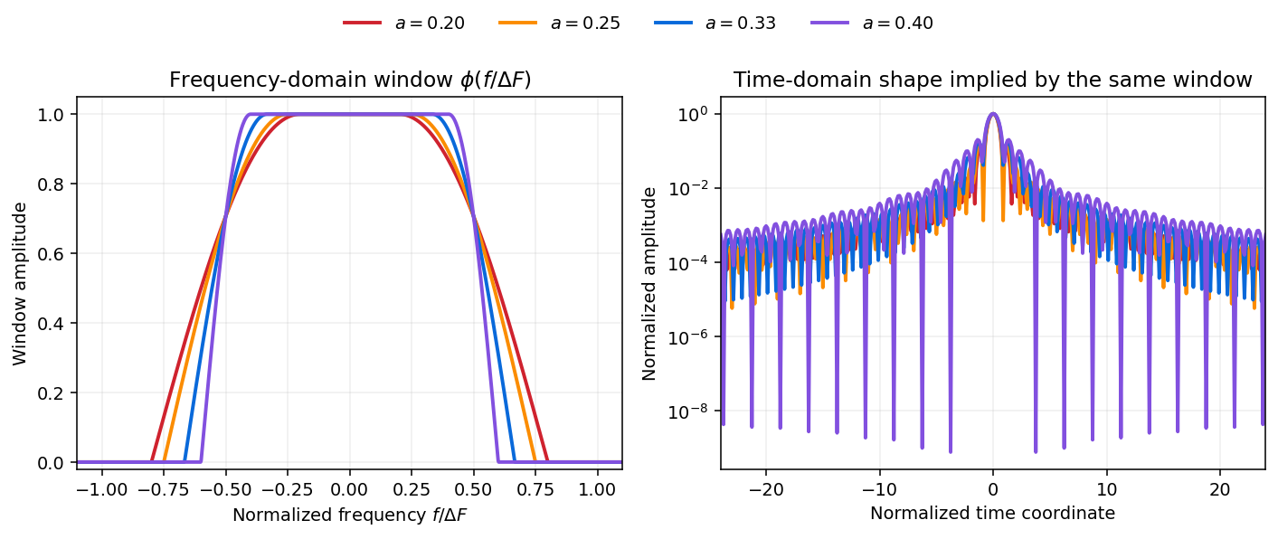
• Left panel: the cosine-tapered \(\tilde\varphi\) shape in normalised frequency coordinates.
• Right panel: the implied time-domain envelope; this is what controls how localised each atom is in time.

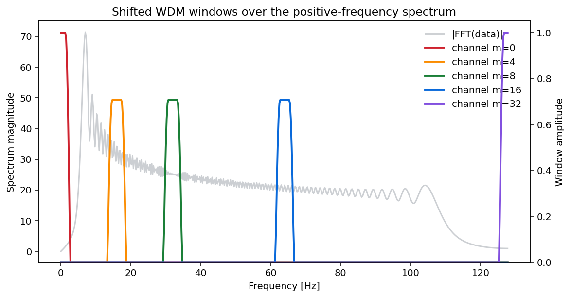
Shifted Windows Define The Channels

The same base window is shifted by \(mN_t/2\) to define each channel \(m\). Adjacent compact Meyer windows overlap and obey a partition-of-unity property, allowing exact reconstruction:

\[ \tilde\varphi^2(f) + \tilde\varphi^2(f - \Delta F) = \frac{1}{\Delta F} \]

across each overlap region.

The Atoms \(\tilde g_{nm}\)

The Wilson-basis atom definition has three cases, matching the packed \((N_t,\, N_f+1)\) storage:

\[ \tilde g_{nm}[\ell] = \frac{1}{\sqrt 2} \begin{cases} e^{-4\pi i n \ell / N_t}\, \tilde\varphi[\ell] & m = 0 \\[2pt] e^{-2\pi i n \ell / N_t}\Big(C_{nm}\, \tilde\varphi[\ell - m N_t/2] + C_{nm}^{*}\, \tilde\varphi[\ell + m N_t/2]\Big) & 0 < m < N_f \\[2pt] e^{-4\pi i n \ell / N_t}\Big(\tilde\varphi[\ell - N/2] + \tilde\varphi[\ell + N/2]\Big) & m = N_f \end{cases} \]

Note the doubled time-shift exponent (\(4\pi\) instead of \(2\pi\)) for the DC and Nyquist edge channels: those channels oscillate at twice the rate in \(n\) because they see both positive and negative frequency copies of the window simultaneously.

The Phase Factor \(C_{nm}\)

The interior channels use an alternating phase factor

\[ C_{nm} = \exp\!\left[i\tfrac{\pi}{4}\,(1 - (-1)^{n+m})\right] = \begin{cases} 1 & n+m \text{ even} \\ i & n+m \text{ odd} \end{cases} \]

This is the Wilson part of the construction: it combines the positive- and negative-frequency windowed atoms at \(\pm m N_t / 2\) into a single real, orthogonal pair. Without \(C_{nm}\) the pairing would not yield real coefficients with the right orthogonality structure.

The forward transform for the interior block can be written compactly as

\[ w_{nm} = \sqrt 2\, (-1)^{nm}\, \Re\!\left[C_{nm}^{*}\, x_m[n]\right] \]

where \(x_m[n]\) is the length-\(N_t\) inverse FFT of the windowed spectral block at channel \(m\). The \((-1)^{nm}\) checkerboard sign is what produces the alternating pattern visible across the coefficient grid.

Why Orthogonality Matters

The interior atoms satisfy

\[ \sum_{\ell} \tilde g_{nm}^{*}[\ell]\, \tilde g_{pq}[\ell] = \delta_{np}\,\delta_{mq} \]

exactly (to machine precision). This means each interior coefficient \(w_{nm}\) measures the projection onto one localised time-frequency pattern, with no leakage from neighbours in the ideal sense. In practice:

• one atom corresponds to one localised time-frequency cell
• coefficients can be read independently
• forward followed by inverse reconstructs the data to floating-point roundoff
• for stationary white noise the coefficient covariance is exactly diagonal; for coloured stationary noise it is approximately diagonal, with off-diagonal correlations decaying rapidly with \(|n - n'|\) and \(|m - m'|\).

The full packed array is overcomplete only at the DC and Nyquist edges, which together carry \(N_t\) redundant real numbers.

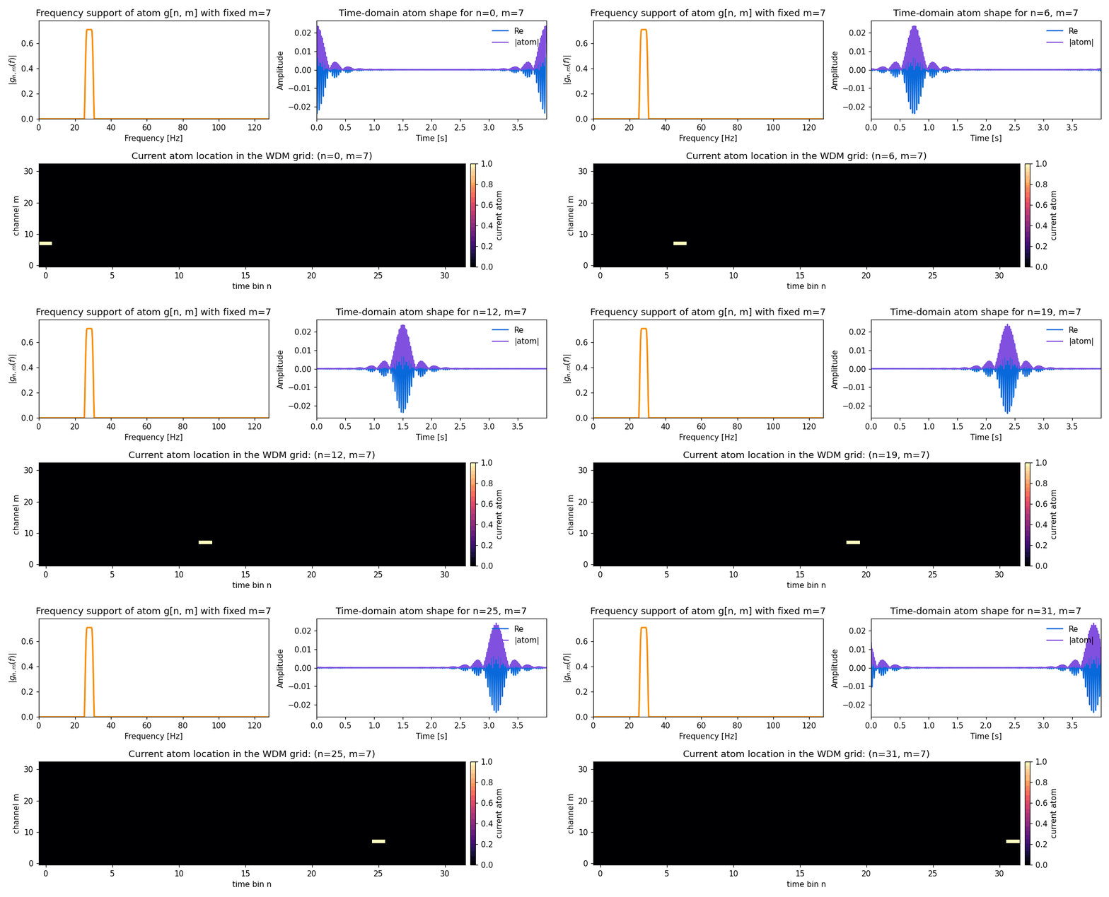
Atom Shift Animation

Keeping one channel fixed and varying \(n\) shifts the atom in time:

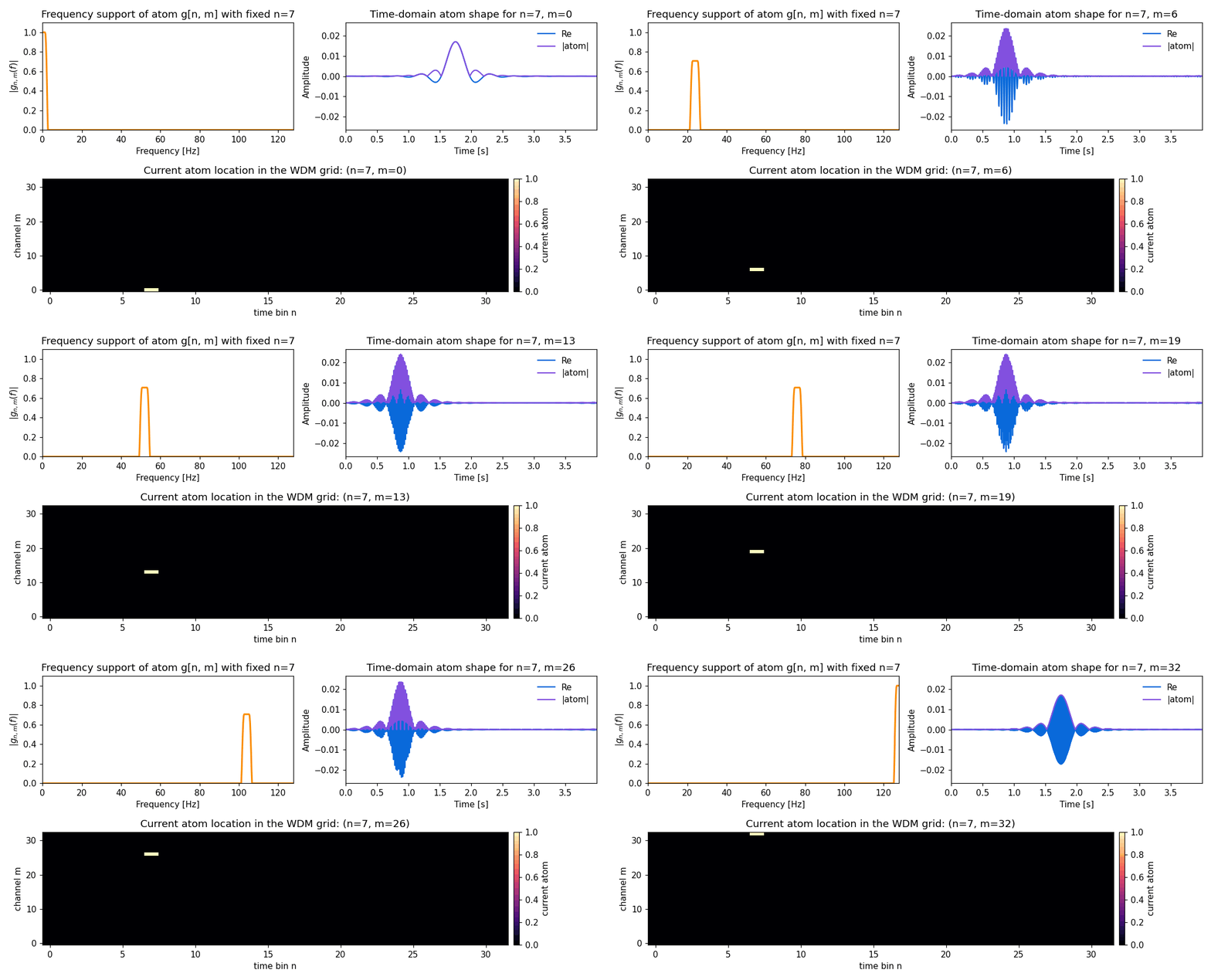
Channel Shift Animation

Keeping one time bin fixed and varying \(m\) shifts the atom in frequency:

So, at a high level:

• changing \(n\) at fixed \(m\) moves an atom in time
• changing \(m\) at fixed \(n\) moves an atom in frequency

Implementation Surface

The shared helpers that define these pieces live in:

• wdm_transform.windows.phi_unit — the dimensionless cosine taper
• wdm_transform.windows.phi_window — \(\tilde\varphi\) as evaluated on the discrete frequency grid
• wdm_transform.windows.cnm — the phase factor \(C_{nm}\)
• wdm_transform.windows.gnmf — the full atom \(\tilde g_{nm}\) in the three-case form above

These helpers preserve their existing Meyer meaning. The separate wdm_transform.windows_gaussian.gaussian_unit and gaussian_window helpers generate the modified-Gaussian samples on the host. For a dimensionless window \(\Phi_\nu\) with channel spacing one, the complete Wilson identity is

\[ \sum_p \Phi_\nu(u+p)\Phi_\nu(u+p+2j)=\delta_{j0}. \]

The package taps \(\sqrt{2/N_t}\,\Phi_\nu(2\ell/N_t)\) therefore have lattice sum \((2/N_t)\delta_{j0}\). Checking only \(j=0\) tests partition of unity; nonzero shifts also need cancellation. Truncating Gaussian spectral support leaves a controlled residual in both this identity and reconstruction.