Choosing Meyer Or Gaussian

Start with Meyer for a fast transform with compact frequency support, particularly when separating narrow frequency features matters. Choose Gaussian when keeping a transient or the influence of a data gap localized in time matters more. Gaussian gains time localization by spreading each atom over a wider frequency range, so the choice depends on your signal and noise.

Both families use the same WDM object and coefficient grid. The Gaussian option implements the orthogonalized modified-Gaussian Wilson window (WDG) from Noah Pearson et al. (2026). It is an orthogonalized window rather than a Gaussian taper applied to the data.

Your priority	Starting choice	Why
Narrow frequency features and small subbands	Meyer	Compact frequency support limits frequency mixing and keeps the required frequency margin small.
Short transients or local effects of gaps	Gaussian	Tighter time localization reduces their spread across nearby time bins.
Lowest transform cost or an existing analysis	Meyer	It is the established default and uses the existing compact kernels.

Compare The Same Signal

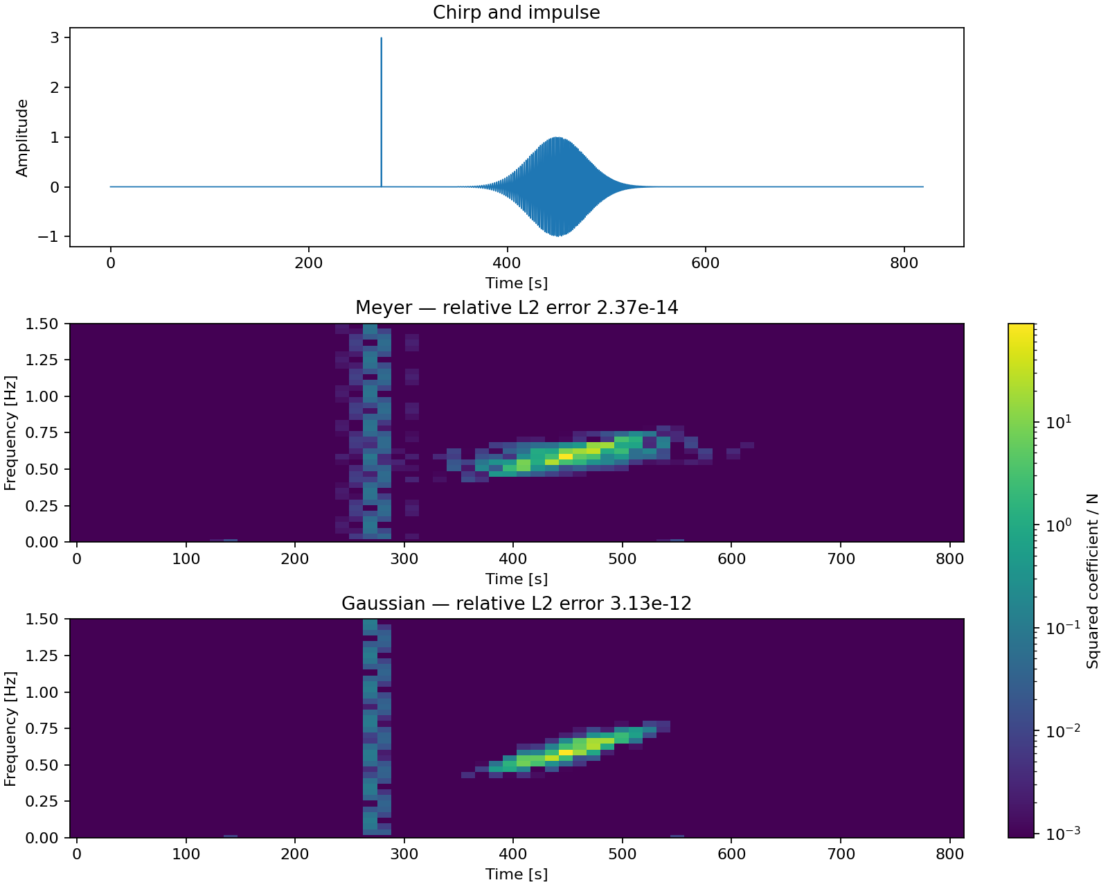
The top panel contains a chirp and an impulse at about 273 seconds. The two maps use the package defaults on the same grid (nt=64, nf=128, dt=0.1 s). They share one logarithmic color scale for squared coefficients divided by N; values below 1e-5 of the shared maximum use the display floor. Compare the impulse's horizontal spread and the chirp's frequency spread to see the tradeoff. Only frequencies from 0 to 1.5 Hz are shown. The runnable example generates the plot and reports relative reconstruction errors of about 2.4e-14 for Meyer and 3.1e-12 for Gaussian.

This compares our default Meyer window (a=1/3, d=1) with default Gaussian (nu=0.5, support=16). The paper's main comparison uses a higher-order Meyer window (d=6), so its reported improvement should not be read as a measured improvement over this package's default.

Switch And Reconstruct

import numpy as np
from wdm_transform import TimeSeries

ts = TimeSeries(np.random.default_rng(42).normal(size=8192), dt=0.1)
meyer = ts.to_wdm(nt=64)  # Meyer remains the default.
gaussian = ts.to_wdm(nt=64, window="gaussian")
recovered = gaussian.to_time_series()

assert (gaussian.window, gaussian.nu, gaussian.support) == ("gaussian", 0.5, 16)
np.testing.assert_allclose(recovered.data, ts.data, atol=1e-10, rtol=1e-10)

The same options work with FrequencySeries.to_wdm, the WDM factories and the four full transform functions. WDM stores the effective window settings and reuses them for both time and frequency inverses. If constructing it from existing coefficients, pass their originating settings. To change family, transform the original series again: changing metadata alone does not convert coefficients to another basis.

Setting	Meyer	Gaussian
Selector	window="meyer" (default)	window="gaussian"
Shape defaults	a=1/3, d=1	nu=0.5
Frequency support	Existing compact window	support=min(16, nf)

Gaussian accepts 0.3 <= nu <= 0.8 and integer 1 <= support <= nf. It rejects nondefault Meyer controls a/d; Meyer rejects Gaussian controls nu/support. Existing calls without a selector keep their previous behavior.

Use Compact Subbands

The compact Fourier-to-WDM, requested-band and inverse APIs support both families with the same window, nu and support options. They take a crop of the one-sided Fourier grid, including DC and Nyquist when those bins are in the crop. Fourier bins outside that crop are treated as zero.

Reuse the same settings for analysis and synthesis. Changing the window variable below switches the whole calculation:

import numpy as np
from wdm_transform.transforms import (
    from_freq_to_wdm_subband,
    from_wdm_to_freq_subband,
)

nt, nf, dt = 64, 128, 0.1
n = nt * nf
window = "gaussian"  # Change to "meyer" to use the original window.
settings = dict(
    df=1.0 / (n * dt),
    nfreqs_fourier=n // 2 + 1,
    nfreqs_wdm=nf,
    ntimes_wdm=nt,
    backend="numpy",  # "jax" uses the same interface.
    window=window,
)
one_sided = np.fft.rfft(np.random.default_rng(7).normal(size=n))
crop_start = 400
crop = one_sided[crop_start:464]
coefficients, first_channel = from_freq_to_wdm_subband(
    crop, kmin=crop_start, **settings
)
reconstructed, first_bin = from_wdm_to_freq_subband(
    coefficients, mmin=first_channel, **settings
)

expected = np.zeros(n // 2 + 1, dtype=complex)
expected[crop_start:464] = crop
np.testing.assert_allclose(
    reconstructed,
    expected[first_bin:first_bin + len(reconstructed)],
    atol=1e-8,
    rtol=1e-10,
)

Gaussian's wider frequency support returns a wider range of channels and reconstructed Fourier bins. The span helpers also accept window, nu and support; use the same settings when planning a crop. To compute only a requested channel block, use from_freq_to_wdm_band.

Subbands return bare arrays and their starting indices, so retain the window settings yourself. Inverse synthesis treats coefficient channels outside the supplied block as zero. Truncating that block further changes the reconstruction. DC/Nyquist reflection and repeated contributions are handled by the compact kernels without allocating the full Fourier spectrum.

Choose Support And Check Your Analysis

support=q retains q half-band spacings on each side of a Gaussian window's frequency center. A spacing is 1/(2*nf*dt), or nt/2 full-FFT bins; the retained window has q*nt taps. More support captures smaller tails and improves reconstruction, while increasing work. It does not change the time grid.

Default nu=0.5, support=16 gave relative reconstruction errors near 3e-12 on the tested float64 grids. In a seeded noise check, support 4/8/16 gave errors near 1e-3, 1e-6 and 3e-12. At nu=0.3, support 16 gave about 7e-8; support 32 reduced that to about 2e-14. Small nf caps the available support. Check the reconstruction error for your chosen grid and parameters rather than assuming the default meets every accuracy requirement.

Gaussian full transforms support NumPy and JAX; the shared CuPy implementation requires validation on a GPU. JAX supports JIT and derivatives with respect to input signals. Gaussian does more frequency gathering and scattering: local warm JAX timings stayed within roughly 3x Meyer, while NumPy synthesis reached about 4.1x. Use wdm_transform_window_benchmark --help to measure your hardware.

Also check your noise model: Gaussian's wider frequency window mixes a wider range of PSD values. The existing wdm_noise_variance channel-center approximation has not been calibrated as a Gaussian colored-noise covariance model. Reconstruction accuracy alone does not validate a diagonal likelihood or quantify the effect of gaps.

Reference: Noah Pearson, Mesut Çalışkan, Sophie Bini and Neil J. Cornish (2026), A compact time-frequency representation for gravitational-wave data analysis, arXiv:2609.05601.