What Is The WDM Domain?
The Wilson–Daubechies–Meyer (WDM) transform is a discrete wavelet-packet time-frequency representation for a one-dimensional sampled signal. It maps \(N\) real samples to a packed grid of \(N\) real coefficients indexed by a time bin \(n\) and a frequency channel \(m\).
It sits between two familiar extremes:
- A time series tells you exactly when something happens, but not in which frequency band.
- An FFT tells you exactly which frequencies are present, but not when they are active.
A short-time Fourier transform partially closes this gap with a sliding window, but imposes a fixed time–frequency resolution across the whole record. The WDM imposes a fixed resolution too, but uses a smooth compactly-supported Meyer window and a Wilson-basis pairing of positive and negative frequencies, yielding exactly orthonormal interior atoms and an exact, closed-form inverse.
The Core Idea
WDM represents the signal with localized atoms \(g_{nm}[\ell]\):
- \(n = 0, \dots, N_t - 1\) indexes a time bin
- \(m = 0, \dots, N_f\) indexes a frequency channel
Each coefficient \(w_{nm}\) measures the projection of the signal onto the atom centred at time bin \(n\) and frequency channel \(m\):
That is why a WDM coefficient grid can be read as a packed time-frequency map.
Why The Grid Has Shape \((N_t,\, N_f + 1)\)
For a signal of length
the transform stores coefficients in a real array of shape \((N_t,\, N_f + 1)\).
The channels are packed as:
- \(m = 0\): DC edge channel — uses a doubled time-shift exponent and no \(C_{nm}\) phase factor
- \(m = 1, \dots, N_f - 1\): interior channels — alternating phase factor \(C_{nm}\) pairs positive- and negative-frequency atoms into a single real Wilson-orthogonal coefficient
- \(m = N_f\): Nyquist edge channel — mirrors the DC construction at the Nyquist frequency
The interior block stores \(N_t (N_f - 1)\) coefficients via the \(C_{nm}\) pairing; the two edge channels each contribute \(N_t\) unpaired real coefficients. The total \(N_t (N_f + 1)\) stored entries represent the same \(N\) time-domain degrees of freedom, with the edge channels overcomplete by exactly \(N_t\) real numbers.
Both \(N_t\) and \(N_f\) must be even.
Orthogonality, Exactly
Unlike many wavelet-packet implementations, the interior WDM atoms \(1 \le m \le N_f - 1\) are exactly orthonormal to machine precision:
This is what makes the WDM domain well behaved for statistical inference: for stationary Gaussian noise the coefficient covariance is approximately diagonal, and the diagonal limit is exact for white noise.
The full packed array including DC and Nyquist is overcomplete by \(N_t\) real numbers — not non-orthogonal. The redundancy lives entirely in the edge channels.
The Inverse Is Closed-Form
Forward followed by inverse returns the original data to floating-point roundoff. The package implements the explicit inverse
with channel-wise formulae for the DC, interior, and Nyquist cases. See Reconstruction and Inference.
Reading The Packed Grid
- Moving horizontally changes the time-bin index \(n\)
- Moving vertically changes the channel index \(m\)
- Bright coefficients indicate that the signal resembles that localized oscillatory atom
In practice, narrow-band features often occupy only a few nearby WDM channels, while transients stay localized in time instead of being smeared across the entire FFT.
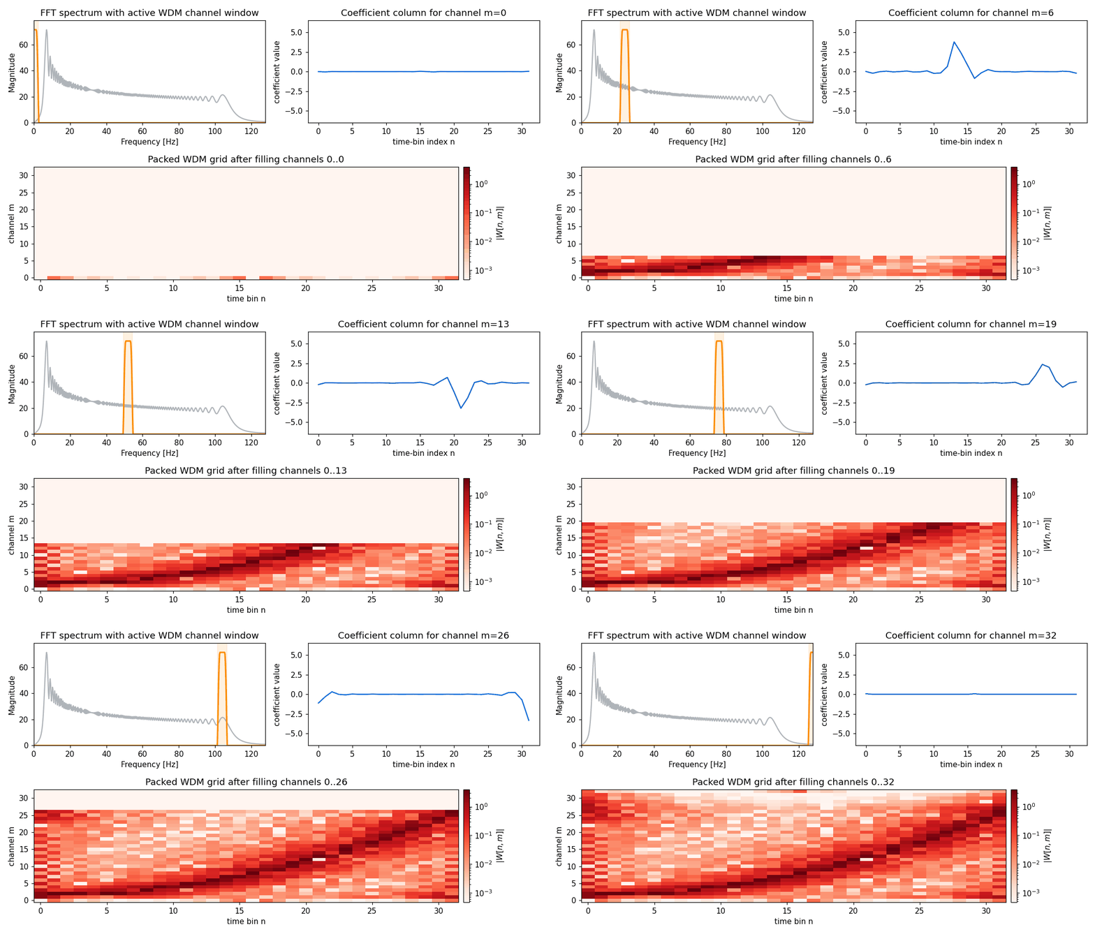
Frequency Packetization Animation
The animation below shows one way to interpret the forward transform:
- start from the FFT of the data
- select one active WDM channel window at a time
- compute the corresponding coefficient column
- fill the packed WDM grid channel by channel
Why This Matters
This view is useful when you want:
- better time localization than an FFT
- a structured coefficient grid that still supports exact reconstruction
- a domain where locally stationary noise has an approximately diagonal covariance, giving a WDM-Whittle likelihood that naturally accommodates slowly-varying spectra
For a full worked example with executable plots, see the walkthrough: