Example

Open In Colab

Example#

Time to Wavelet#

Let’s transform a time-domain signal (of length \(N\)), to the wavelet-domain (of shape \(N_t\times N_f\)) and back to time-domain.

! pip install pywavelet -q
Hide code cell content
from scipy.signal import chirp
import numpy as np
from typing import List
import matplotlib.pyplot as plt

from pywavelet.types import TimeSeries
from pywavelet.transforms import from_time_to_wavelet, from_wavelet_to_time


def generate_chirp_time_domain_signal(
    t: np.ndarray, freq_range: List[float]
) -> TimeSeries:
    fs = 1 / (t[1] - t[0])
    nyquist = fs / 2
    fmax = max(freq_range)
    assert (
        fmax < nyquist
    ), f"f_max [{fmax:.2f} Hz] must be less than f_nyquist [{nyquist:2f} Hz]."

    y = chirp(
        t, f0=freq_range[0], f1=freq_range[1], t1=t[-1], method="hyperbolic"
    )
    return TimeSeries(data=y, time=t)


def plot_residuals(ax, residuals):
    ax.hist(residuals, bins=100)
    # add textbox of mean and std
    mean = residuals.mean()
    std = residuals.std()
    textstr = f"$\mu={mean:.1E}$\n$\sigma={std:.1E}$"
    props = dict(boxstyle="round", facecolor="wheat", alpha=0.5)
    ax.text(
        0.05,
        0.95,
        textstr,
        transform=ax.transAxes,
        fontsize=14,
        verticalalignment="top",
        bbox=props,
    )
    ax.set_xlabel("Residuals")
    ax.set_ylabel("Count")
    ax.ticklabel_format(axis="x", style="sci", scilimits=(0, 0))
    return ax


# Sizes
dt = 1 / 512
Nt, Nf = 2**6, 2**6
mult = 16
freq_range = (10, 0.2 * (1 / dt))
ND = Nt * Nf

# time grid
ts = np.arange(0, ND) * dt
h_time = generate_chirp_time_domain_signal(ts, freq_range)


# transform to wavelet domain
h_wavelet = from_time_to_wavelet(h_time, Nf=Nf, Nt=Nt, mult=mult)

# transform back to time domain
h_reconstructed = from_wavelet_to_time(h_wavelet, dt=h_time.dt, mult=mult)

# Plots
fig, axes = plt.subplots(1, 4, figsize=(18, 4))
_ = h_time.plot_spectrogram(ax=axes[0])
_ = h_wavelet.plot(ax=axes[1], absolute=True, cmap="Reds")
_ = h_reconstructed.plot_spectrogram(ax=axes[2])
_ = plot_residuals(axes[3], h_time.data - h_reconstructed.data)
axes[0].set_title("Original Time Domain")
axes[1].set_title("Wavelet Domain")
axes[2].set_title("Reconstructed Time Domain")
axes[3].set_title("Residuals")
for ax in axes[0:3]:
    ax.set_ylim(*freq_range)
fig.savefig("roundtrip_time.png")
plt.close()

Provide data as a TimeSeries/FrequencySeries object

These objects will ensure correct bins for time/frequency in the WDM-domain.
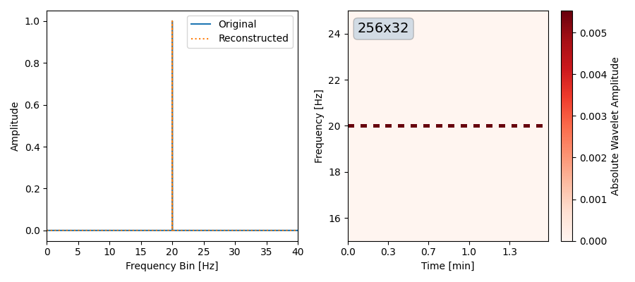
Freq to Wavelet#

This time, we use a sine-wave in the frequency domain.

import numpy as np
from pywavelet.types import FrequencySeries
from pywavelet.transforms import from_freq_to_wavelet, from_wavelet_to_freq
import matplotlib.pyplot as plt

f0 = 20
dt = 0.0125
Nt = 32
Nf = 256
N = Nf * Nt

freq = np.fft.rfftfreq(N, dt)
hf = np.zeros_like(freq, dtype=np.complex128)
hf[np.argmin(np.abs(freq - f0))] = 1.0


h_freq = FrequencySeries(data=hf, freq=freq)
h_wavelet = from_freq_to_wavelet(h_freq, Nf=Nf, Nt=Nt)
h_reconstructed = from_wavelet_to_freq(h_wavelet, dt=h_freq.dt)


fig, axes = plt.subplots(1, 2, figsize=(9, 4))
_ = h_freq.plot(ax=axes[0], label="Original")
_ = h_wavelet.plot(ax=axes[1], absolute=True, cmap="Reds")
_ = h_reconstructed.plot(ax=axes[0], ls=":", label="Reconstructed")
axes[1].set_ylim(f0 - 5, f0 + 5)
axes[0].legend()
fig.savefig("roundtrip_freq.png")
plt.close()